$$ \gdef\dx{\mathrm{d}x} \gdef\dm{\mathrm{d}m} \gdef\dr{\mathrm{d}r} $$
$\gdef\dx{\mathrm{d}x}$ $\gdef\dm{\mathrm{d}m}$ $\gdef\dr{\mathrm{d}r}$
Intro
Last time, in Part I, we covered the basic concepts leading up to random variables and their distributions. In this post, things will start to get cracking as we build up to the law of the unconscious statistician, the law of large numbers, and Monte Carlo integration. Along the way, we’ll introduce the following terms:
| Term | Notation |
|---|---|
| Expected Value of $X$ under distribution $p$ | $\mathbb{E}_p[X]$ |
| Variance of $X$ under distribution $p$ | $\mathbb{V}_p[X]$ |
Expected Value
The expected value $\mathbb{E}_p[X]$ of a random variable $X$ with distribution $p$ is the probability-weighted average of its possible values. Intuitively, it represents the average value we would observe over many independent repetitions of the same experiment.
For a discrete random variable:
The sum is taken over all possible values $x$ of $X$. Here, $p(x)$ is the probability mass function (PMF) $p_X(x)$, the probability that $X=x$.
For a continuous random variable:
The integral is taken over all possible values $x$ of $X$. Here, $p(x)$ is the probability density function (PDF) $f_X(x)$, the probability density at $x$.
Note: The expected value of a contant $c\in\mathbb{R}$ is the constant itself.
The constant $c$ can be thought of as a discrete random variable that takes the value $c$ with probability $1$.
$$
\mathbb{E}[c]=c
$$
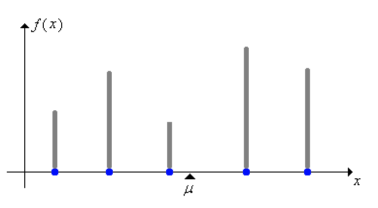
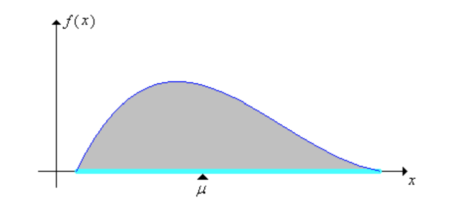
The expected value of $X$ is also called the mean of the distribution of $X$ and is frequently denoted $\mu$. In physics, the mean is the center of mass, the balance point.
Moment
The moment of $X$ about $a \in \mathbb{R}$ of order $n \in \mathbb{N}$ is defined as $$ \mathbb{E}\big[ (X-a)^n \big] $$
| Moments about $0$ are referred to as moments, or raw moments. | $ \mathbb{E}[ X^n ]$ |
| Moments about $\mu = \mathbb{E}[X]$ are referred to as central moments. | $\mathbb{E}\big[ (X-\mu)^n \big]$ |
Note that the first central moment is always $0$, as
We will revisit moments when we discuss variance.
Example: Fair Die
Let’s get the expected value of a fair die roll.
First, let $S=T=\lbrace 1,2,3,4,5,6 \rbrace$ and define our random variable $X : S \to T$ as an identity mapping. The measurement $X(s) = s $ is simply the number rolled.
Since the die is fair, the PMF $p(x) = \dfrac{1}{6}$ for each possible value of $x$. The expected value is:
Although we can’t actually roll the value $3.5$, it represent the average value we would approach over many indepedent rolls.
Example: Weighted Die
Now let’s say we’re gambling for money, and higher rolls win. To give give ourselves a little bit of a unfair advantage, we bring out a weighted die where the probability of rolling a $6$ is twice as likely as rolling any of the other numbers.
The expected value is then:
So our weighted die has an expected value of approximately $3.86$, a little higher than the fair die’s expected value of $3.5$.
Example: Dart throw
Now let’s look at the expected value of a continuous random variable. We’re going to reuse the dart throwing experiment from part 1, where a dart lands uniformly over the area of a circular target of radius $R$. The random variable $X$ measures the distance from the bullseye, and we’ve already derived the PDF $p(r)$ as:
The expected value $\mathbb{E}_p[X]$ is calculated as follows:
So on average, we would expect the dart to land two-thirds of the way from the center to the edge.
Law of Large Numbers
If we sample from the distribution of $X$, that is re-run the same experiment independently, we create a sequence of random variables $(X_1, X_2, \dots)$ each with the same distribution as $X$. The sample mean $\overline{X}_n$ after $n$ runs is:
$$ \overline{X}_n = \frac{1}{n} \sum _{i=1}^n X_i $$
$\overline{X}_n$ is itself a random variable, whose realized value is the average of the realized values of $X_1, \dots, X_n$.
The law of large numbers (LLN) informally states that as the number of samples increases, the sample mean converges to the expected value.
Law of the Unconscious Statistician
The law of the unconscious statistician (LOTUS) is a theorem for finding the expected value of a function $g$ of a random variable $X$. It is so named because people often use it without consciously realizing that it requires a theorem.
Applying $g$ to $X$ produces another random variable $g(X)$, which has its own probability distribution. However, the distribution of $g(X)$ is not needed: LOTUS shows us that the expected value $\mathbb{E}[g(X)]$ can be computed using only the distribution of $X$.
The discrete case with PMF $p_X$ is:
And the continuous case with PDF $f_X$ is:
Variance
The variance of $X$ is defined as the second central moment of $X$, where $\mu = \mathbb{E} [ X ]$:
If $X$ is discrete with PMF $p_X$, then:
If $X$ is continuous with PDF $f_X$, then:
Variance is often denoted as $\sigma^2$, and its positive square root, standard deviation, as $\sigma$.
Aside: Moment of Inertia
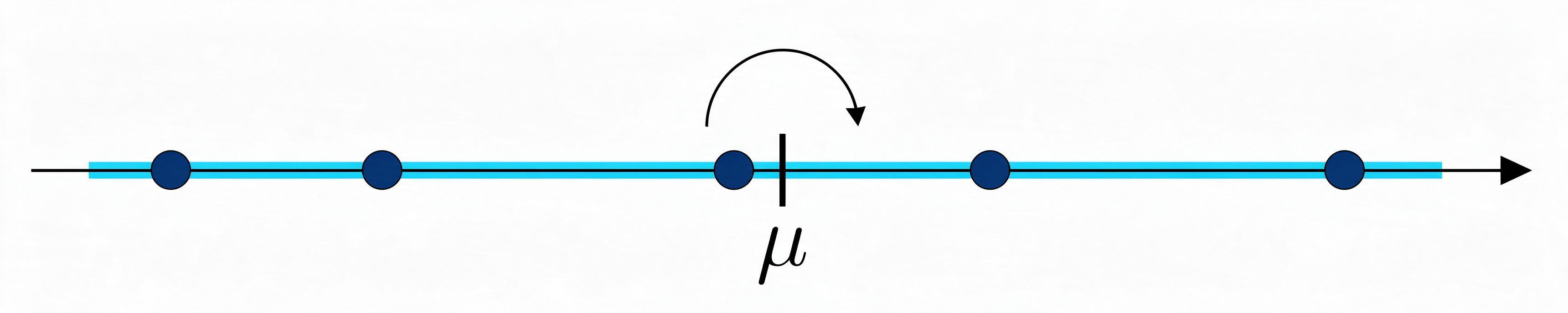
In physics, the moment of inertia $I_\mu$ of a mass distribution along a line measures its resistance to rotation about its center of mass $\mu$.
where:
| Quantity | Expression |
|---|---|
| Position | $x$ |
| Differential mass | $\dm=\rho(x) \thinspace \dx$ |
| Mass density | $\rho(x)$ |
| Differential width | $\dx$ |
For the probability analogue, normalize the mass density by its total mass to obtain a PDF:
| Quantity | Expression |
|---|---|
| Total mass | $M = \int \rho(x) \thinspace \dx$ |
| $f_X(x) = \dfrac{\rho(x)}{M}$ |
Then, the variance is equal to the moment of inertia divided by total mass:
Sneak peek for the 3D inertia tensor, after normalizing the mass density into a PDF:
Monte Carlo Integration
It’s time for the big boy, Monte Carlo integration!
Monte Carlo techniques use repeated random sampling, and are so named after the famous Casino de Monte-Carlo in Monaco. Monte Carlo integration is a clever technique that rewrites an integral as an expected value, and approximates it with a sample mean.
Derivation
We want to estimate the integral $I$ of a function $f$:
$$ I = \int f(x) \thinspace \dx. $$
Do we have anything in our toolbox that contains an integral of a function?
We do! By LOTUS, the expected value of a function $g(X)$ is:
$$
\mathbb{E}_p\left[g(X)\right] = \int g(x) \thinspace p(x) \thinspace \dx
$$
Let’s set that expected value equal to $I$.
$$ \mathbb{E}_p\left[g(X)\right] = \int g(x) \thinspace p(x) \thinspace \dx = \int f(x) \thinspace \dx = I $$
Now we have a relationship between $g$, $f$, and $p$: $$ g(x) \thinspace p(x)=f(x). $$
Solving for $g$, we can rewrite our expected value in terms of the function $f$ we’re trying to integrate, and any PDF $p$ that can sample where $f$ is nonzero. We no longer need $g$.
$$ \mathbb{E}_p\left[\frac{f(X)}{p(X)}\right] = \int f(x) \thinspace \dx = I. $$
Now the LLN informally tells us that the sample mean converges to the expected value.
Define the single-sample random variable
$$ \widehat{I}^{(1)} = \frac{f(X)}{p(X)} , \qquad \mathbb{E}_p\left[\widehat{I}^{(1)}\right] = I. $$
Then draw independent samples $(X_1, \dots, X_n)$ from $p$. Each sample gives an independent single-sample estimate:
$$ \widehat{I}_i^{(1)} = \frac{f(X_i)}{p(X_i)}. $$
Their sample mean converges to $I$:
This gives us the full definition of Monte Carlo integration
Example: Sum of a vector
Say we want to compute the sum $S$ of the numbers in a vector $$ v=( 10, 13, 43, 74, 25 ) $$
$$ S = \sum_{k=1}^{5} v_k $$
We could use a simple loop,
#include <array>
#include <iostream>
#include <numeric>
int main()
{
    const std::array v { 10, 13, 43, 74, 25 };
    const int S { std::accumulate( v.begin(), v.end(), 0 ) };
    std::cout << "S = " << S << '\n';
}
S = 165
but that’s stupid. We want to do this with Monte Carlo integration, with a million samples.
The Monte Carlo estimator also works for finite sums.
The random variable $X$ is uniform over $(1, 2, 3, 4, 5)$, so its distribution is $$ p(X_i)=\frac{1}{5}. $$
Here, $v_{X_i}$ is a random element of the vector $v$, selected using the random sample index $X_i$. Thus our estimator becomes:
Then our code becomes
#include <array>
#include <iostream>
#include <numeric>
#include <random>
#include <span>

float EstimateSum( std::span< const int > v, const int n = 1000000 )
{
   std::default_random_engine rng{ 0 };
   std::uniform_int_distribution< int > X{ 0, ( int )v.size() - 1 };

   int result{};
   for( int i{}; i < n; ++i )
      result += v[ X( rng ) ];

   return ( 5.0f / n ) * result;
}

int main()
{
    const std::array v { 10, 13, 43, 74, 25 };
    const float S { EstimateSum( v ) };
    std::cout << "S is approximately equal to " << S << '\n';
}
S is approximately equal to 164.873
Example: $\int_0^\pi \sin(x) \thinspace \mathrm{d}x$
Let’s find an estimator $\widehat{I}^{(n)}$ for the integral
$$ \widehat{I}^{(n)} \approx \int_0^\pi \sin(x) \thinspace \dx $$
According to Monte Carlo integration, we can estimate an integral by averaging the values $\dfrac{f(X_i)}{p(X_i)}$.
We already have $f(x) = \sin(x)$, the function we want to integrate. We need to draw samples $X_i$ from a random variable $X$ with an appropriate PDF $p$. We’ll let $X$ be uniformly distributed on the integration bounds $[0, \pi]$, so its PDF is $$ p(x) = \frac{1}{ \pi }. $$
Samples $X_i$ are easy to generate: draw a uniform random number from $0$ to $\pi$.
The estimator is thus:
The intuition is that, because $p$ is uniform, our estimator approximates the area under the curve as the width of the interval times the average height of the function.
#include <cmath>
#include <iostream>
#include <numbers>
#include <random>

float EstimateIntegral( const int n = 1000000 )
{
   std::default_random_engine rng{ 0 };
   std::uniform_real_distribution< float > X{ 0, std::numbers::pi_v< float > };

   float result{};
   for( int i{}; i < n; ++i)
      result += std::sin( X( rng ) );

   return ( std::numbers::pi_v<float> / n ) * result;
}

int main()
{
   std::cout << "Integral estimate: " << EstimateIntegral() << std::endl;
}
Integral estimate: 2.00179
Coming up next
We now have the basic structure for Monte Carlo integration. In part 3 we will look at sampling using the inversion method and importance sampling.