Intro
Computer graphics often involves estimating complicated lighting integrals using Monte Carlo integration. This requires a background in random numbers and probability. By the end of this post you should understand the basics of probability, including the following terms and notations:
| Term | Notation |
|---|---|
| Outcome | $s$ |
| Set of Outcomes | $S$ |
| Event | $A$ |
| Event Space | $\mathcal{S}$ |
| Probability Measure | $\mathbb{P}$ |
| Sample Space | $(S, \mathcal{S})$ |
| Probability Space | $(S, \mathcal{S}, \mathbb{P})$ |
| Random Variable | $X$ |
| Probability Distribution of $X$ | $\mathbb{P}_X$ |
| Probability Mass Function (PMF) | $p_X$ |
| Cumulative Distribution Function (CDF) | $F_X$ |
| Probability Density Function (PDF) | $f_X$ |
Example: Rolling a die
Let’s roll a fair six-sided die.
Outcome
An outcome $s$ represents the result of an experiment.
- Before rolling, it could be one of many possible results
- After rolling, we observe the realized outcome, ie $s=5$.
Set of Outcomes
The set of outcomes $S$ contains all possible outcomes $s$.
$$ S = \lbrace 1,2,3,4,5,6 \rbrace $$
$$ s \in S $$
We assume each outcome is equally likely, with probability $\dfrac{1}{6}$.
Event
An event $A$ is a subset of possible outcomes. $$ A \subseteq S $$ For example:
| $A = \lbrace 1, 3, 5 \rbrace$ | event for “rolled an odd number” |
| $B = \lbrace 5, 6 \rbrace$ | event for “rolled a 5 or higher” |
| $C = \lbrace 6 \rbrace$ | event for “rolled a 6” |
If the realized outcome is $s=5$, events $A$ and $B$ occurred, and $C$ did not.
$$ s \in A $$ $$ s \in B $$ $$ s \not\in C $$
Note that event $A$ occurs exactly when $s \in A$.
In this die example, we take each subset of $S$ to be an event.
| The full event $S$ always occurs | $s \in S$ |
| The empty event $\emptyset$ never occurs | $s \not\in \emptyset$ |
Event Space
The event space $\mathcal{S}$ is the collection of all measurable subsets of $S$ that we treat as events. It’s a set of sets. In this die example, we take: $$ \mathcal{S} = 2^S $$
$2^S$ means “power set of S”, which is the set of all subsets of $S$.
It contains $A$, $B$, $C$, $S$, $\emptyset$, and every other subset of $S$.
In fact, the number of events is $|\mathcal{S}| = 2^{|S|} = 2^6 = 64$ events.
Probability Measure
A probability measure $\mathbb{P}$ assigns a probability to each event in the event space.
$$ \mathbb{P} : \mathcal{S} \to [0,1] $$
The probability assigned to the entire set of outcomes $S$ is $1$
$$ \mathbb{P}(S) = 1 $$
In the example of rolling a single die, we had the events
| $A = \lbrace 1, 3, 5 \rbrace$ | event for “rolled an odd number” |
| $B = \lbrace 5, 6 \rbrace$ | event for “rolled a 5 or higher” |
| $C = \lbrace 6 \rbrace$ | event for “rolled a 6” |
The probabilities assigned by the probability measure $\mathbb{P}$ are:
For mutually exclusive events, the probability of their union is the sum of their probabilities. For example:
Sample Space
The sample space $(S, \mathcal{S})$ of an experiment is the set of outcomes $S$ together with the event space $\mathcal{S}$.
Under other conventions, the term sample space is used to refer to just the set of outcomes $S$. However, here we will continue to distinguish the set of outcomes $S$ from the sample space $(S, \mathcal{S})$.
Probability Space
The probability space $(S, \mathcal{S}, \mathbb{P})$ is the triple consisting of the set of outcomes $S$, the event space $\mathcal{S}$, and the probability measure $\mathbb{P}$.
A short recap following our terminology:
| $S$ | Set of outcomes |
| $\mathcal{S}$ | Event space |
| $\mathbb{P}$ | Probability measure |
| $(S, \mathcal{S})$ | Sample space |
| $(S, \mathcal{S}, \mathbb{P})$ | Probability space |
Before we go into random variables, let’s go through a couple of examples.
Examples
Example: 1 coin flip
Let’s flip a fair coin.
Example: 2 coin flips
Let’s flip a fair coin twice. The two flips are independent, that is the result of the first flip $s_1$ does not influence the result of the second flip $s_2$.
The set of outcomes $S^{(2)}$ has four possible outcomes:
where an outcome $s^{(2)}$ records the ordered pair of flip results, $s_1$ and $s_2$ $$ s^{(2)} = (s_1, s_2) \in S^{(2)} $$
And the event that the $i$-th flip was heads is given by
$$ A_i^{(2)} = \Big\lbrace ( s_1, s_2) \in S^{(2)} : s_i \in A^{(1)} \Big\rbrace , i = 1, 2 $$
| $A_1^{(2)} = \Big\lbrace ( H, H ), ( H , T) \Big\rbrace$ | event for “the first flip was heads” |
| $A_2^{(2)} = \Big\lbrace ( H, H ), ( T, H ) \Big\rbrace$ | event for “the second flip was heads” |
For example if the realized outcome was heads followed by tails, then:
Example: N coin flips
Random Variable
A probability space $(S, \mathcal{S}, \mathbb{P})$ models an experiment by specifying possible outcomes, events, and their probabilities. A random variable is a measurement of interest in that experiment. For example:
- the sum of two dice rolls
- the number of heads in several coin flips
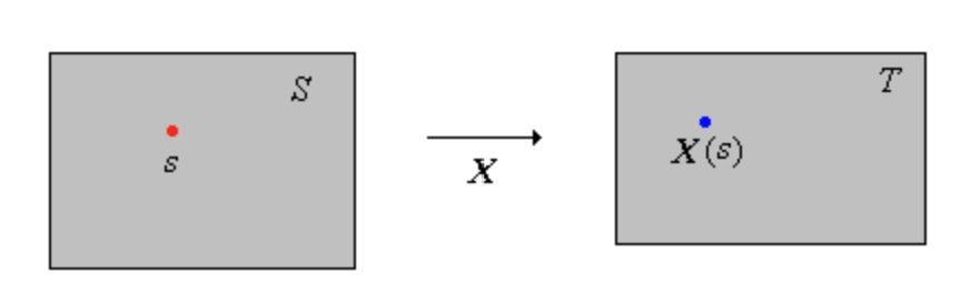
Mathematically, a random variable $X$ is a function that maps outcomes $s \in S$ to $X(s) \in T$. $$ X:S \to T $$ Although random variables are functions, probability notation often leaves the argument implicit, writing simply $X$ rather than $X(s)$. The realized value of $X$ depends on the outcome. When $s \in S$ occurs, $X$ takes on the realized value $X(s) \in T$.
For a measurable set of values $B \subseteq T$, the corresponding preimage event $X^{-1}(B)$ in $S$ is written:
$$ \lbrace X \in B \rbrace = X^{-1}(B) = \lbrace s \in S: X(s) \in B \rbrace $$
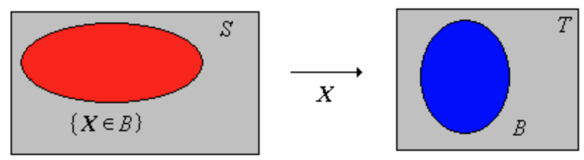
A random variable $X$ must be measurable, that is the preimage of each measurable set of values $B \subseteq T$ must be an event in $\mathcal{S}$.
$$ X^{-1}(B) \in \mathcal{S} $$
Example: # of heads in 2 coin flips
Let $X$ be the number of heads in two coin flips. Here let’s use 0 for tails and 1 for heads.
The outcome $s$ is the ordered pair
$$ s = (s_1, s_2) \in S = \lbrace 0, 1 \rbrace ^2 $$
$X$ counts the number of heads $$ X(s) = s_1 + s_2 $$
The full mapping is
where
$$ S = \lbrace 0, 1 \rbrace ^ 2 = \Big\lbrace ( 1, 1 ), (1, 0), (0, 1) , (0,0) \Big\rbrace $$
$$ T = \lbrace 0, 1, 2 \rbrace $$
In this example
- $S$ is the set of outcomes from flipping two coins
- $T$ is the set of possible values (measurements) of $X$
The values of $X$ are given by:
Note that $X(1,1) = 2$ is shorthand for $X\big((1,1)\big)=2$.
Notation examples
- If $x \in T$, then
- $\lbrace X = x \rbrace = \Big\lbrace X \in \lbrace x \rbrace \Big \rbrace = \lbrace s \in S : X(s) = x \rbrace$
- If $X$ is real-valued, and $a,b \in \mathbb{R}$, and $a<b$, then
- $\lbrace a \leq X \leq b \rbrace = \Big\lbrace X \in [ a, b ] \Big \rbrace = \lbrace s \in S : a \leq X(s) \leq b \rbrace$
- If $T \subseteq \mathbb{R}^k$, then $X$ is a random vector with each component a real-valued random variable $X_i$
- $X=(X_1, X_2, \dots, X_k)$
- The outcome itself can be thought of a random variable. Let $T=S$ and let $X$ be the identity function. Then:
- $X(s) = s$
- $\lbrace X \in A \rbrace = A$
Probability Distribution
Recall that a random variable $X:S \to T$ maps outcomes to measurements.
The probability distribution $\mathbb{P}_X$ of $X$ assigns each measurable set of values $B \subseteq T$ a probability $\mathbb{P}_X(B)$ describing how likely $X$ is to fall within $B$.
The probability distribution $\mathbb{P}_X$ is in itself a probability measure. The difference is:
- probability measure $\mathbb{P}$ assigns probabilities to events in $S$,
- probability distribution $\mathbb{P}_X$ assigns probabilities to measurable sets of values in $T$
$$ \mathbb{P}_X( B ) = \mathbb{P}( X \in B ) = \mathbb{P}( X ^ {-1} ( B ) ) $$
Recall from earlier, for a measurable set of values $B \subseteq T$, the corresponding preimage event $X^{-1}(B)$ in $S$ is written:
$$ \lbrace X \in B \rbrace = X^{-1}(B) = \lbrace s \in S: X(s) \in B \rbrace $$
The preimage of $B$ under $X$, written as $X ^ {-1} ( B )$, is an event to which $\mathbb{P}$ can assign a probability.
Probability Distribution Example
Let’s take another look at the two-coin flip example. The random variable $X$ counts the number of heads, so the measurement $X(s)$ is the number of heads in the observed outcome $s$.
Here, we are interested in the probability that we get at most one head. In other words, we are interested in the probability that this measurement belongs to the set $B = \lbrace 0, 1 \rbrace \subseteq T$. The probability distribution $\mathbb{P}_X$ assigns to this set the probability $\mathbb{P}_X$.
To calculate this probability, first let’s look at which outcomes produce a measurement in $B$. The set of outcomes $S$ is:
$$ S = \big \lbrace (0,0), (0,1), (1,0), (1,1) \big \rbrace $$
The outcomes with at most one head form the the event $A \subseteq S$, which is the preimage of $B$ under $X$.
$$ A = X ^ {-1} ( B ) = X ^ {-1} \big( \lbrace 0, 1 \rbrace \big) = \big\lbrace (0,0), (1,0), (0,1) \big\rbrace $$
Since the four outcomes are equally likely, and three of them belong to $A$, we get:
Discrete Random Variable
The random variable $X$ representing the number of heads in two coin flips is an example of a discrete random variable. A discrete random variable $X$ has a countable image (range). In this case, there are 4 outcomes $s$ in the set of outcomes $S$, and 3 possible measurements in the range $X(S)$:
$$ S=\lbrace (0,0), (0,1), (1,0), (1,1) \rbrace $$
$$ X(S) = \lbrace 0, 1, 2 \rbrace $$
Probability Mass Function
The probability mass function (PMF) $p_X$ is the function that gives the probability $p_X(x)$ for a given value $x$ in the range $X(S)$.
$$ p_X(x) = \mathbb{P}(X=x) = \mathbb{P}_X(\lbrace x \rbrace) $$
The distribution $\mathbb{P}_X$ assigns probability to a set $B$ by summing $p_X$ over the values in the set:
$$ \mathbb{P}_X(B) = \sum _{x \in B \cap X(S) } p_X(x) $$
For example: $$ \mathbb{P}_X( \lbrace 0, 1 \rbrace ) = p_X(0) + p_X(1) = \frac{1}{4} + \frac{1}{2} = \frac{3}{4} $$
Cumulative Distribution Function
The cumulative distribution function (CDF) $F_X$ of a random variable $X$ is the function that gives the probability that the random number $X$ is at or below a given value $x$ $$ F_X(x) = \mathbb{P}(X \le x ) = \mathbb{P}_X \big( ( -\infty, x] \big) $$
Continuing the two-coin flip example
Note that $ \mathbb{P}_X( \lbrace 0, 1 \rbrace ) = F_X(1)$
Continuous Random Variable
On the other hand, a continuous random variable can take on an uncountable number of values. For example, a dart lands uniformly at random over the area of a circular dartboard of radius $R$ (we are ignoring the skill aspect of throwing darts here). Let the random variable $X$ represent the distance the dart lands from the bullseye.
| Outcome $s = (u,v)$ | Where the dart lands |
| Random variable $X$ | Function measuring distance from center |
| Measurement $X(s) = \sqrt{u^2 + v^2} $ | Observed distance |
Then $$ S = \big \lbrace (u,v) : u^2 + v^2 \leq R^2 \big \rbrace $$
$$ X(S) = [0,R] $$
Let’s start with the cumulative distribution function $F_X$. Recall that the cumulative distribution function gives the probability that a random variable $X$ is at or below a given value. Here $F_X$ will give the probability that the dart is less than or equal to a distance $r$ from the center. $$ F_X(r) = \mathbb{P}( X \le r ) = \frac{\text{area of inner circle}}{\text{area of outer circle}} = \frac{\pi r^2}{\pi R^2} = \frac{ r^2}{ R^2}, 0 \le r \le R $$
Probability Density Function
The probability density function (PDF) $f_X$ of a continuous random variable $X$ is the function that gives the probability density $f_X(x)$ of a given value $x$ in the range $X(S)$, the probability per unit $x$.
Unlike a PMF $p_X$, which gives the probability of an exact value of a discrete random variable, the PDF $f_X$ gives probability density, not the probability of an exact value.
For a random variable $X$ with PDF $f_X$: $$ \mathbb{P}(X=x) =0 \quad \text{ for every } x $$
Integrating the probability density function $f_X$ over an interval $[a,b]$ gives the probability that $X$ falls within that interval.
$$ \mathbb{P}(a \le X \le b) = \int_a^b f_X(x) dx $$
At points where the PDF $f_X$ is continuous, it is the derivative of the CDF $F_X$:
$$ \frac{d}{dx} F_X(x) = f_X(x) $$
In our dart throwing example, for $0 < r < R$:
Thus the PDF $f_X$ of $X$ is:
From $f_X$, you can see that the dart is more likely to land in an outer ring than an inner ring of the same thickness, as outer rings have more area.